02 / SENSING

Sensing and perception

The useful output is a registered scene: geometry, water quality, motion, and detection signals tied to a surface position—not a single magical sensor. This page treats every optical, acoustic, and electromagnetic number as a candidate engineering envelope that must be calibrated in the water where it will be used.

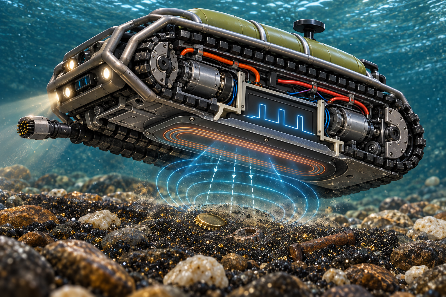
GoldRiverBot concept illustration

The active-stereo camera module

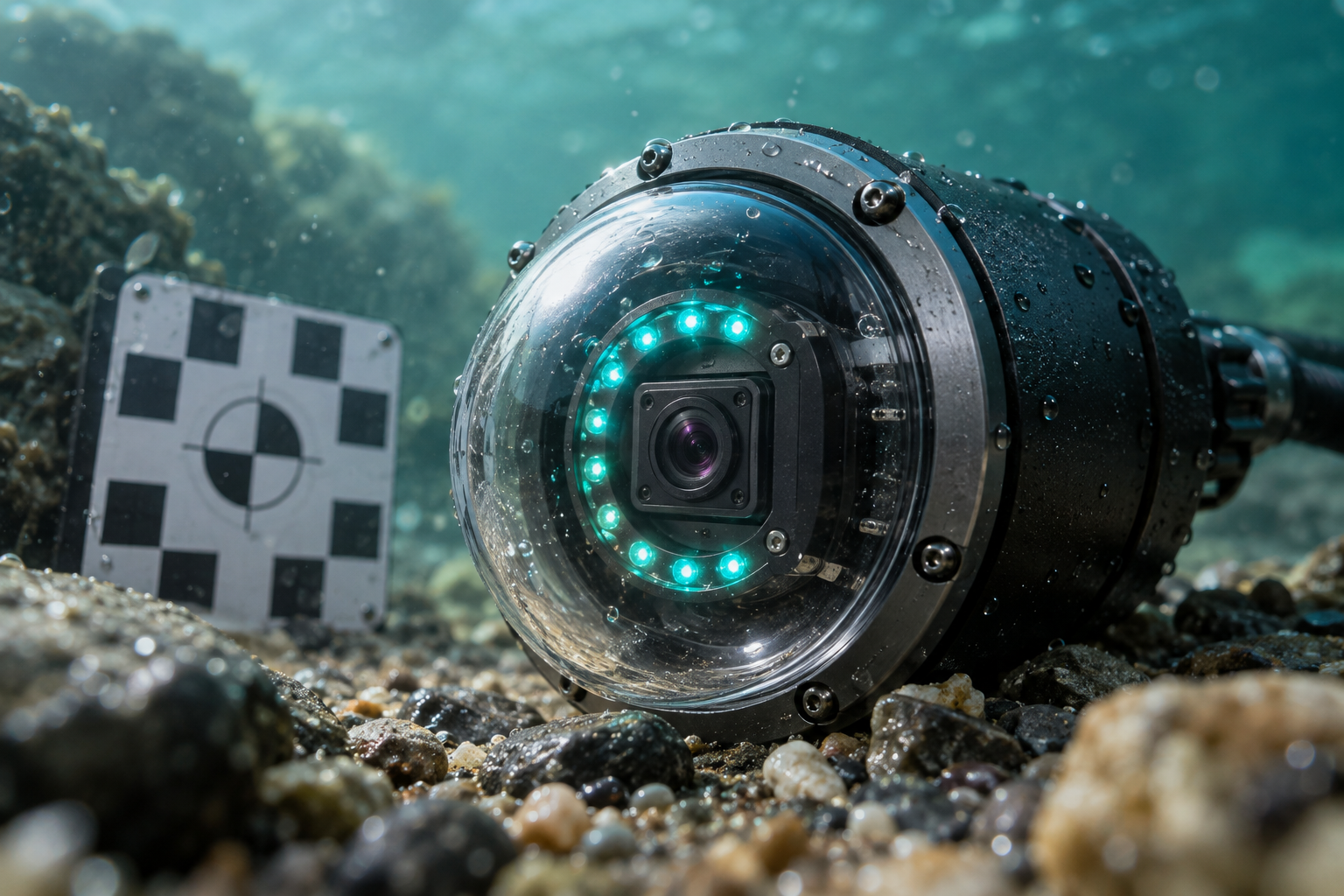
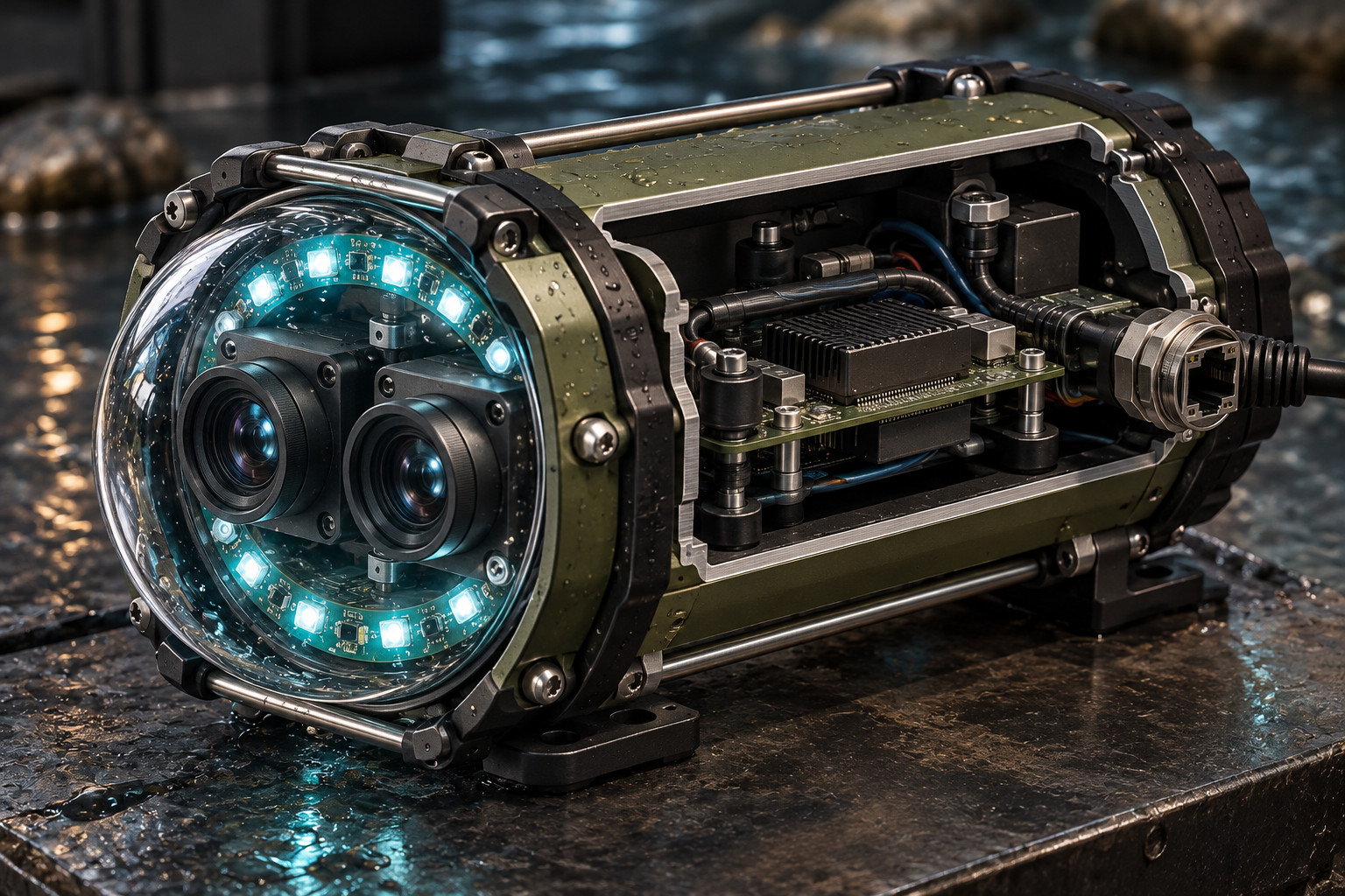
Two synchronized global-shutter sensors capture the same instant from slightly different viewpoints. The edge computer matches features between the pair, estimates disparity, and turns it into a local depth map. Global shutters reduce the skew that rolling shutters introduce when the crawler moves over rocks or the current shakes the housing. The proposed module uses a pressure-rated dome, a blue-green light ring, short-range focus, and a serviceable Ethernet/PoE connector.

Sensor class
Dual global shutter, 1–12 MP candidate range
Frame rate
30–60 fps research target
Viewport
Dome or Aquagon-style refractive correction
Link
Gigabit Ethernet / PoE concept
Working view
Recessed low-front pair, roughly 15–35° down
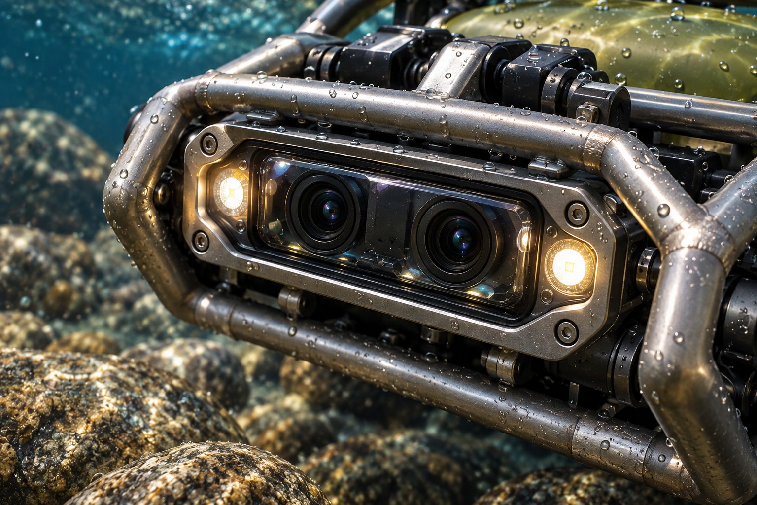
The active-stereo camera module

Why water changes the camera problem

Water absorbs red light quickly and scatters suspended silt. The useful blue-green window is roughly 400–550 nm, so the camera and light ring should be designed around that band rather than assuming daylight color will survive. A second macro camera can work at 5–50 cm for the collection tray, but focus, backscatter, and calibration targets matter more than headline megapixels. UV fluorescence and active IR structured light are experimental options—not guaranteed gold signatures or universal depth solutions.

Blue-green window
Approx. 400–550 nm
UV research band
Approx. 300–400 nm; corrosion/ions only
Active IR
Approx. 750–850 nm; test in actual turbidity
Macro range
Conceptually 5–50 cm
Why water changes the camera problem

Water correction and computer vision

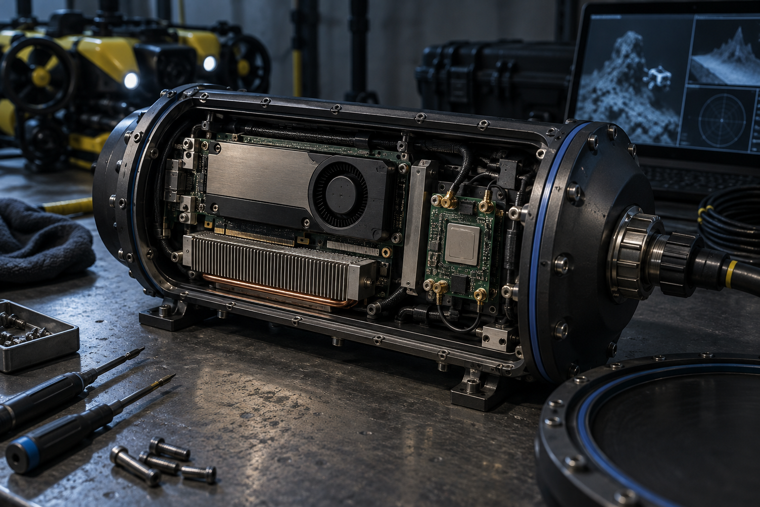
Sea-thru- or WaterGAN-inspired processing can estimate wavelength-dependent attenuation and reduce the blue-green cast before a detector sees the frame. That is a preprocessing hypothesis, not a license to manufacture detail that was never captured. A customized YOLOv8 or YOLOv10-style model could be trained on bedrock cracks, black-sand lines, coins, chains, and representative geology. The model should report calibrated confidence and an abstain state; a shiny pebble or pyrite must remain a possible false positive.

  • Store raw frames beside every corrected frame.
  • Train on site-specific geology and lighting, not internet stock images.
  • Use confidence calibration, hard negatives, and an explicit unknown class.
Water correction and computer vision

Green LiDAR: a conditional detail layer

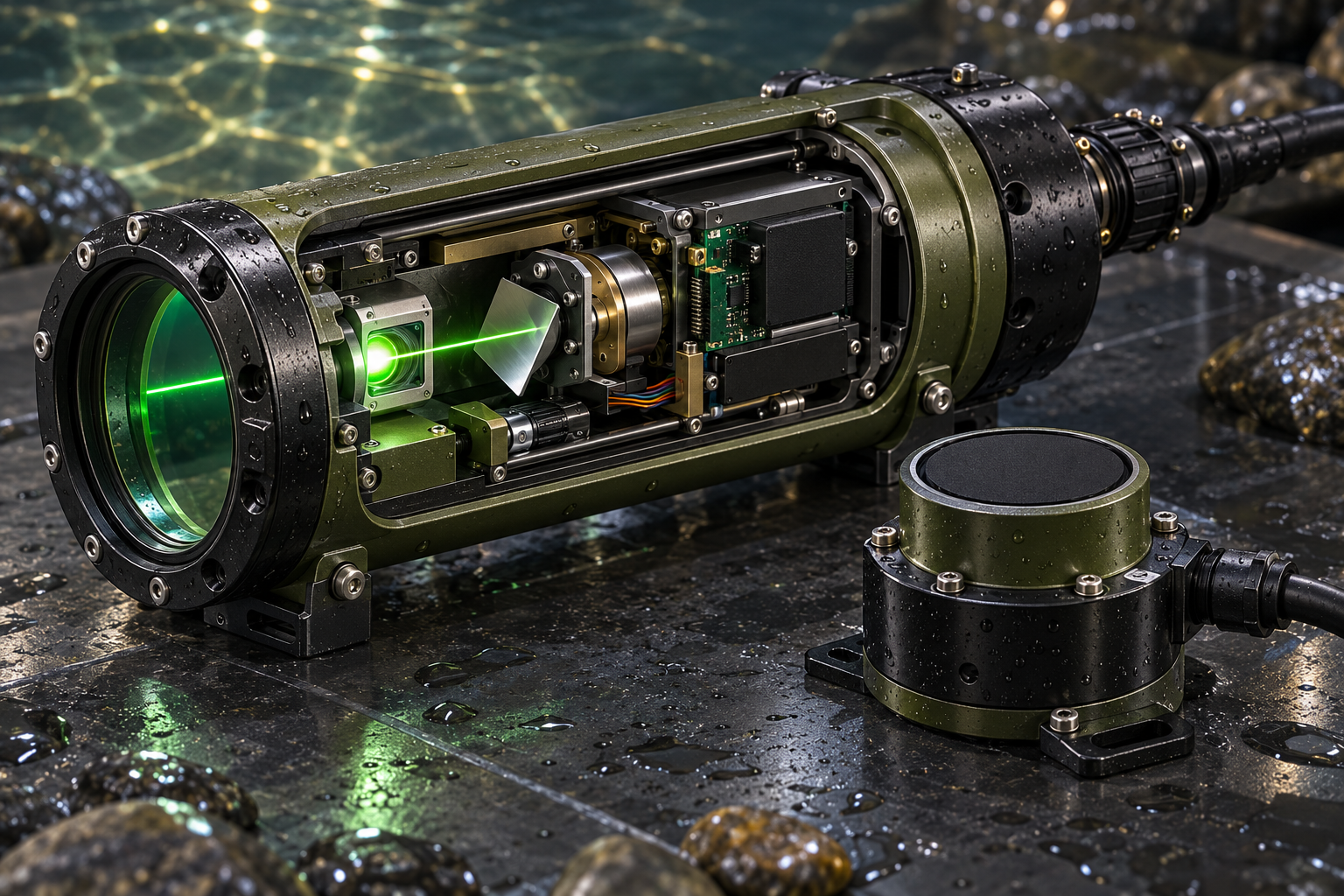
Bathymetric or subsea LiDAR uses green light near 532 nm because that wavelength can travel farther through clear shallow water than infrared. A scanning mirror and time-of-flight electronics can produce a dense local point cloud, but bubbles and turbidity quickly shorten range. Premium bathymetric systems may use dual-pulse surface/bed returns to correct water level and refraction; a small crawler would more likely use a compact experimental scanner and rely on depth/IMU calibration. Terrestrial 1064 nm IR LiDAR is not a drop-in underwater sensor.

Optical wavelength
532 nm green-light concept
Best case
Clear, shallow water and close-range structure
Failure modes
Silt, bubbles, surface glare, refraction
Role
Fine geometry after sonar finds the area
Green LiDAR: a conditional detail layer

Sonar is the robust baseline

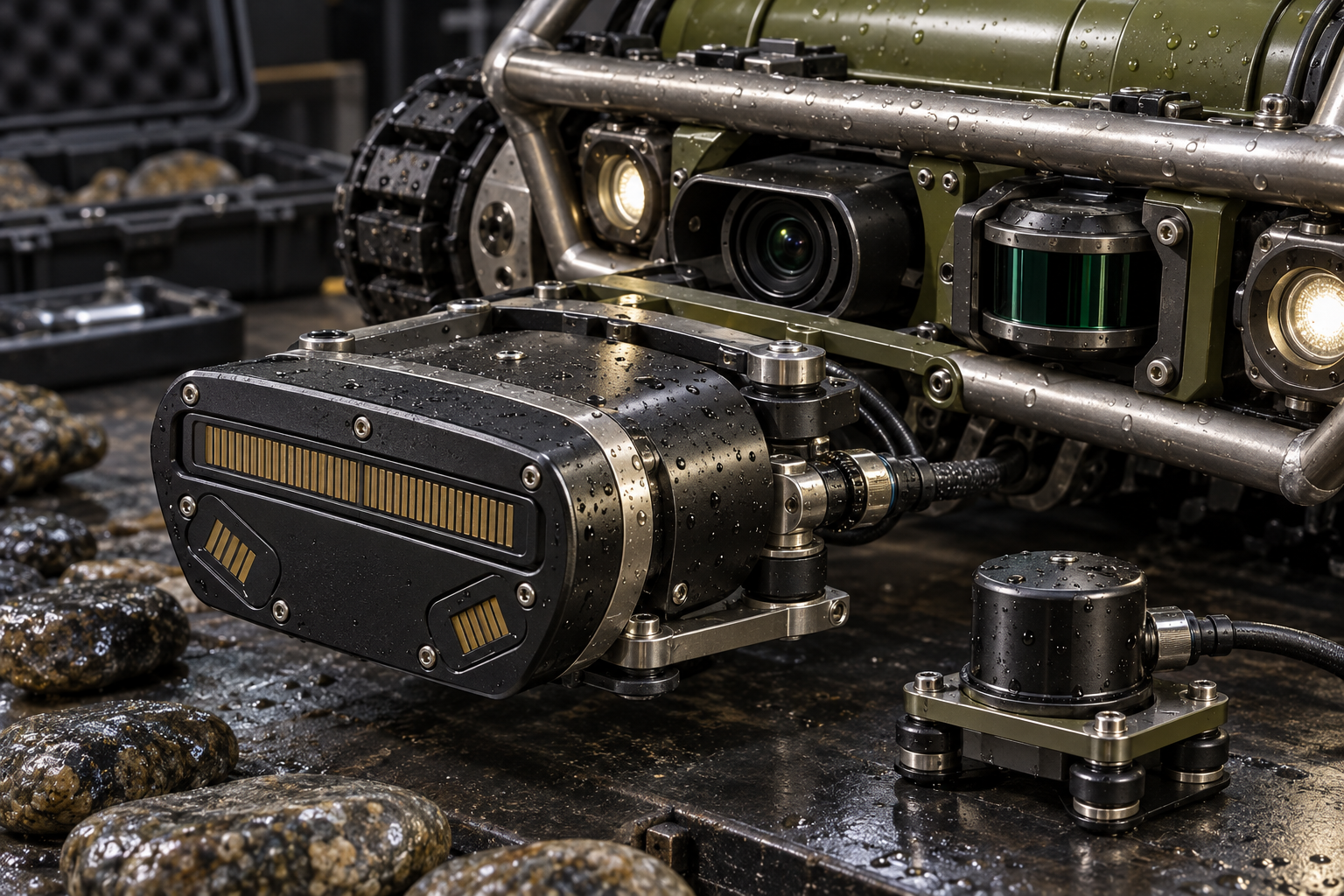
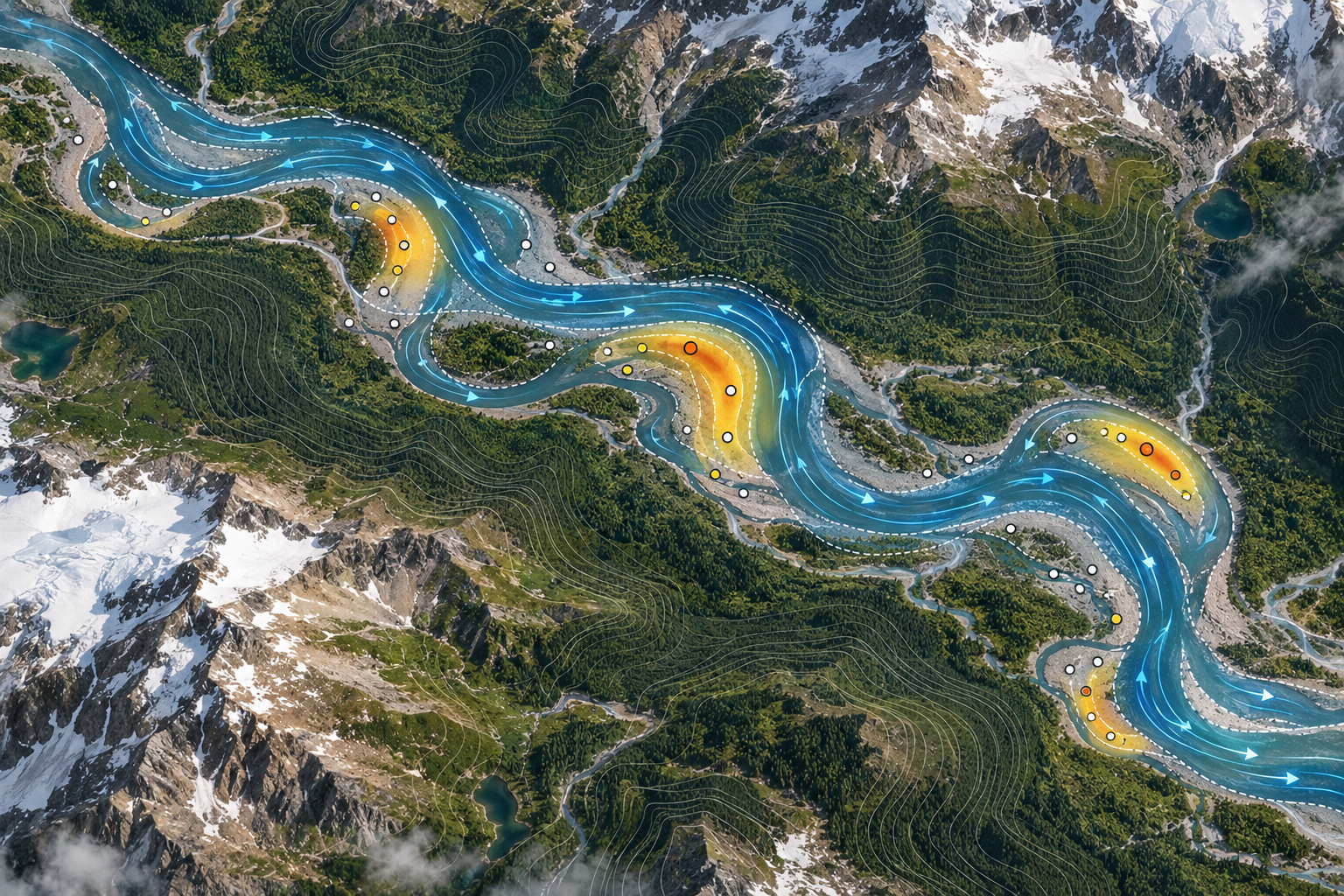
Forward-looking or multibeam sonar supplies the primary obstacle and morphology layer when optical systems lose contrast. Acoustic returns can identify the silhouette of a logjam, boulder, ledge, or undercut bank even when the camera sees only suspended particles. The fusion engine should register sonar range/angle with stereo depth, IMU attitude, depth, and track odometry, then retain the uncertainty instead of flattening every return into a crisp-looking image.

  • Sonar-first route planning in turbid water.
  • Optical stereo for near-field texture and sample positioning.
  • Conditional LiDAR for high-detail geometry in clear water.
Sonar is the robust baseline

Pulse induction detector

The PI coil sends a high-current pulse, waits for the transmit field to collapse, and samples one or more receive windows in the decay curve. An initial laboratory sweep might explore approximately 100–1,000 pulses per second and pulse widths from tens to hundreds of microseconds. PI is attractive in mineralized or saline conditions because it does not require the same continuous ground-balance behavior as VLF, but it has minimal discrimination: a conductive iron fragment, aluminum, or steel can look like a target. Tiny sub-gram flakes remain a difficult sensitivity case.

Signal
Transient decay / conductivity anomaly
Initial sweep
100–1,000 pulses/s research range
Pulse width
Tens to hundreds of microseconds
Trade-off
Depth and stability versus discrimination
Pulse induction detector

The sensor-fusion record

A target should be interesting because multiple independent observations agree: LiDAR or sonar finds a narrow trap, stereo sees a bedrock texture or black-sand line, PI records a repeatable conductive response, and the surface buoy supplies a coordinate with known offset. The resulting event stores raw sensor windows, calibration state, timestamp, depth, pose covariance, and a confidence grade. It should say ‘repeat here’ rather than ‘gold found’ until the cartridge and laboratory result support that claim.

  • Raw + corrected imagery
  • Sonar returns and point-cloud confidence
  • PI waveform and repeated-pass comparison
  • GNSS buoy position, tether offset, and uncertainty
  • Cartridge ID and chain-of-custody link
The sensor-fusion record

Calibration and test gates

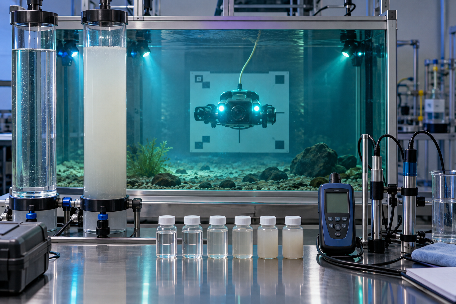
Before a river mission, the camera needs a geometric calibration target behind the dome, the LiDAR needs a range/refraction check, sonar needs a known reflector, and PI needs known conductors plus mineralized-background trials. Run the full stack in clear water, then add controlled turbidity, bubbles, moving illumination, and representative cobble. Acceptance is measured false-alert rate, localization error, dropout behavior, and safe fallback—not a single attractive demo frame.

  • Bench → pressure vessel → clear-water tank → turbidity tank → permitted river
  • Record temperature, depth, turbidity, and lighting with every test
  • Keep an operator review path for every autonomous target
Calibration and test gates